SigComm 2022 Cosmos Testbed Tutorial

Labrador Group

In this tutorial we'll demonstrate how to run a basic wireless experiment using software defined radios in the COSMOS testbed. Two COSMOS nodes will be used: one to transmit a signal, and the other to receive it.

Resources Used

For this example we'll use two USRP b210 SDRs on ​grid. These SDRs have a USB connection to a PC, which is the device you're loading the orbit image onto and connecting to over ssh. They also have an fpga connected to the four antennas. We won't have to worry about the specifics of the USRP for this tutorial but you can look at the links on ​this page for more information.

Tutorial Setup

Follow the steps below to gain access to the console and set up your node with an appropriate image.

1. Use ssh to connect to the console for the grid domain:

   ssh your-username@console.grid.orbit-lab.org
   

   NOTE: typically when using the testbed, you will have to reserve the domain you wish to use on the ​scheduler page. We have already made the reservation for you.

2. Use OMF commands to load the baseline-uhd.sdr image on your resources.

OMF is a command line utility that is run from the console in order to manage nodes: turn them on and off, save the contents of the hard disk as an "image", and load saved images back onto them.

In this case, we're loading the "baseline-sdr.ndz" image, which is a pre-built image provided for researchers to use as a starting point. The image contains UHD 3.15 and Gnuradio 3.8 and uses Ubuntu 18.04.

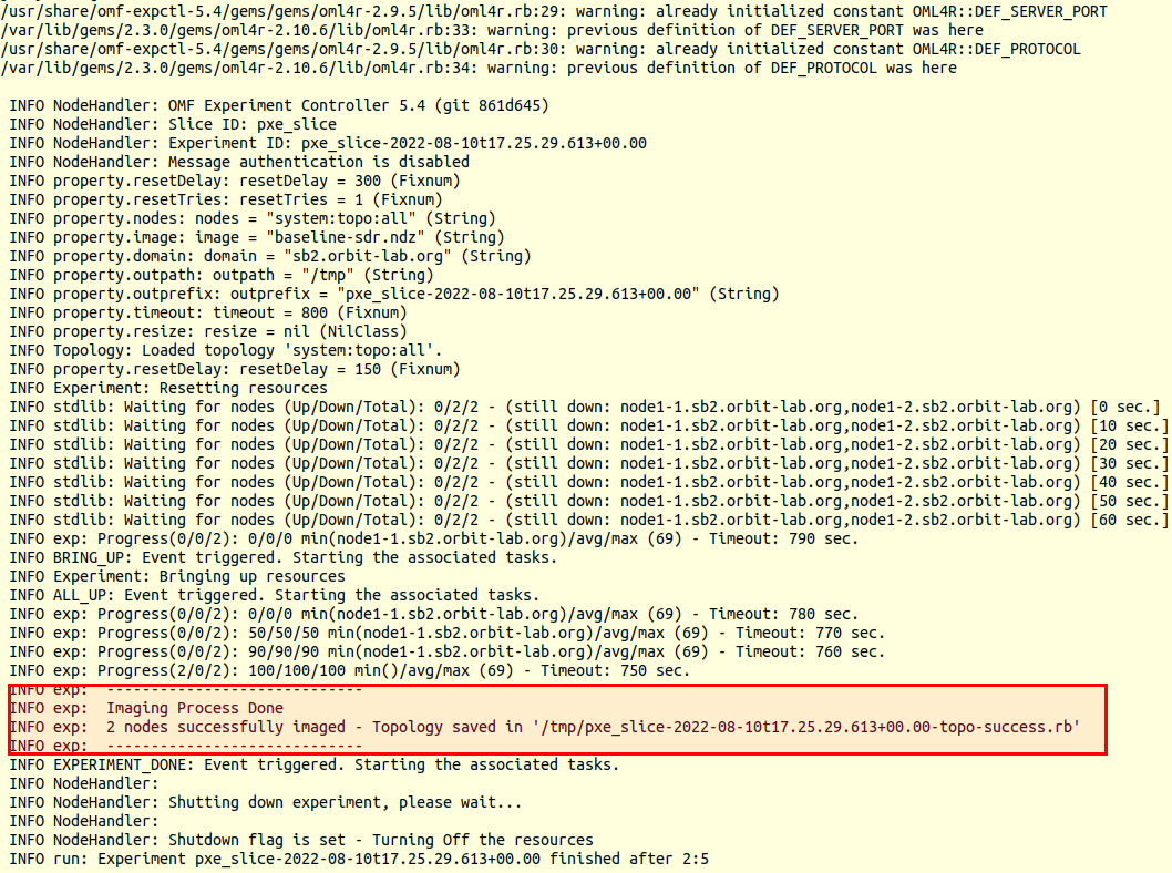
omf load -i baseline-sdr.ndz -t node3-2,node8-7

This is a good opportunity to look at the output of the image loading process. At first glance, it can look like a lot of text, but there is some useful information there to help you understand what is going on. Here is the output of running the above command:

We can see from this output that the image loading process has two phases: the first, noted in red, in which OMF is waiting for the nodes to boot up and load a client which will receive the omf image data and write it to disk; and the second, noted in blue, in which OMF actually performs the imaging process. This output shows a successful imaging process— we can tell because of the text noted in pink, which says that the imaging process is done and there were two nodes successfully imaged. The filename displayed there will contain a list of all the nodes which were successfully imaged.

Once in a while, you may see an imaging process where some or all of the nodes fail to image. This can happen because something goes wrong either in the first step (a node fails to boot up and register with the imaging process) or in the second step (the node fails to load the image onto its hard disk). If there is a failure, it will be noted in the output at the end of the imaging process— there will be additional files listed for nodes that fail to check in, and nodes in which imaging failed.

Always check the output to make sure that your nodes were successfully imaged.

3. Once the nodes are successfully imaged, turn them on and check the status

   omf tell -a on -t node3-2,node8-7
   

   omf stat -t node3-2,node8-7
   

4. After waiting for the nodes to power up and boot, you will be able to ssh to them from the console:

   ssh root@node3-2
   

Experiment Execution

Configure and detect the radio

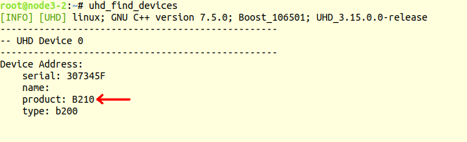
1. Use uhd_find_devices to make sure that the onboard b210 SDR is detected:

Notice that running this command with no arguments will sometimes detect other SDR resources in the testbed which are reachable over the network. We can ignore those for now and focus just on the onboard b210.

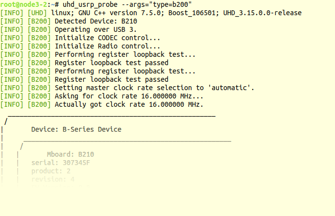
2. Use the uhd_usrp_probe command to get more details on the b210. Specifying type=b200 ensures only the directly connected radio is probed, instead of the radios on the network.

Run the experiment

For this demo, we'll be running some of the demo applications that are installed with uhd. Source code for all of the samples can be found here: ​https://github.com/EttusResearch/uhd/tree/UHD-3.15.LTS/host/examples

1. ssh to node3-2 and start the rx_ascii_art_dft demo with the following command:

   /usr/lib/uhd/examples/rx_ascii_art_dft --args "type=b200" --freq 2400e6 --rate 5e6 --frame-rate 10 --gain 10 --ref-lvl -30 --dyn-rng 70
   

   Note that we are looking at the frequency band around 2.4GHz. You should see an output like this:

2. ssh to node8-7 and start the tx_waveforms demo with the following command:

   /usr/lib/uhd/examples/tx_waveforms --args="type=b200" --wave-freq 1e6 --wave-type SINE --freq 2400e6 --rate 5e6 --gain 10 --ampl 0.2
   

As we can see from the arguments passed to the application, we are transmitting a 1MHz sine wave as a signal using 2.4GHz as the carrier frequency. On the DFT visualization on sdr2-md1, you should see a peak representing the transmitted signal:

We can generate a different type of signal by changing the wave-type argument. For instance, if we transmit a square wave:

/usr/lib/uhd/examples/tx_waveforms --args="type=b200" --wave-freq 1e6 --wave-type SQUARE --freq 2400e6 --rate 5e6 --gain 10 --ampl 0.2

We can see that the spectrum of the received signal now contains multiple peaks. This is the result of the spectral characteristics of a square wave.

Both tx_waveforms and rx_ascii_art_dft can take --help as a command line argument, which will display the lists of arguments that you can provide and what each argument does. There are also a number of other demo applications in the /usr/lib/uhd/examples directory, which you can take a look at.