Description

Geo2SigMap is an efficient framework for high-fidelity RF signal mapping leveraging geographic databases, ray tracing, and a novel cascaded U-Net model. The project offers an automated and scalable pipeline that efficiently generates 3D building and path gain (PG) maps. The ​repository is split into two distinct partitions:

• Scene Generation: A pure Python-based pipeline for generating 3D scenes for arbitrary areas of interest.
• ML-based Propagation Model: ML-based signal coverage prediction using our pre-trained model based on the cascaded U-Net architecture described in ​this paper.

As of November 2025, v2.0.0 enhances the scene generation pipeline to include:

• LiDAR Terrain Data
• Building Height Calibration using Digital Elevation Models (DEMs)

This drastically improves the accuracy of the environment being processed by the ML-based Propagation Model or a ray tracer of your choice. Throughout our ​Jupyter Notebook examples, we utilize Sionna RT. This package is open-source and popular for creating coverage predictions. If you are unfamiliar with Sionna RT, feel free to read Nvidia's ​Technical Report to better understand how it works. Tutorials for Sionna can be found ​here.

Prerequisites

To use Geo2SigMap with ease, we strongly suggest managing python packages using Anaconda. Anaconda's package manager, ​conda, offers everything you need with no extra configuration.

The installation process should ensure that all required packages are installed. In the event of any issue, this is the ​pipreqs list as of 1/21/2025:

osmnx >= 2.0.0
numpy
pyproj
shapely
rasterio
tqdm
pillow
open3d

Given the large overhead for ray tracing and ML tasks, access to a dedicated GPU (with RT cores) is also suggested. Using Sionna RT with a CPU offers limited performance and will restrict the capabilities for experimentation.

Package Installation

1. Create the Conda Environment:

conda create --yes --name g2sm --channel conda-forge pdal python=3.12
conda activate g2sm
pip install pyvista==0.45.2

If you opt not to use conda, please note the additional installation of pyvista v0.45.2

2. Clone and Install geo2sigmap:

git clone https://github.com/functions-lab/geo2sigmap
cd geo2sigmap/package
pip install .

The package is now installed and can be called via the CLI tool or using the Python function API.

Creating a Scene

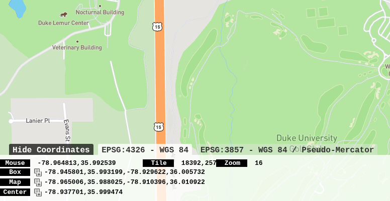
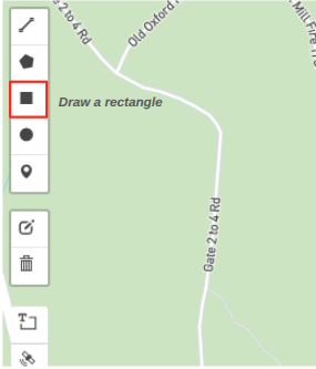
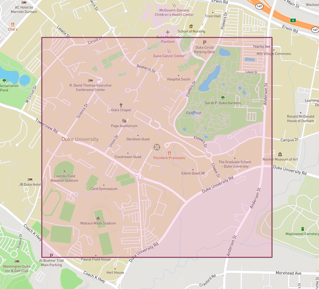
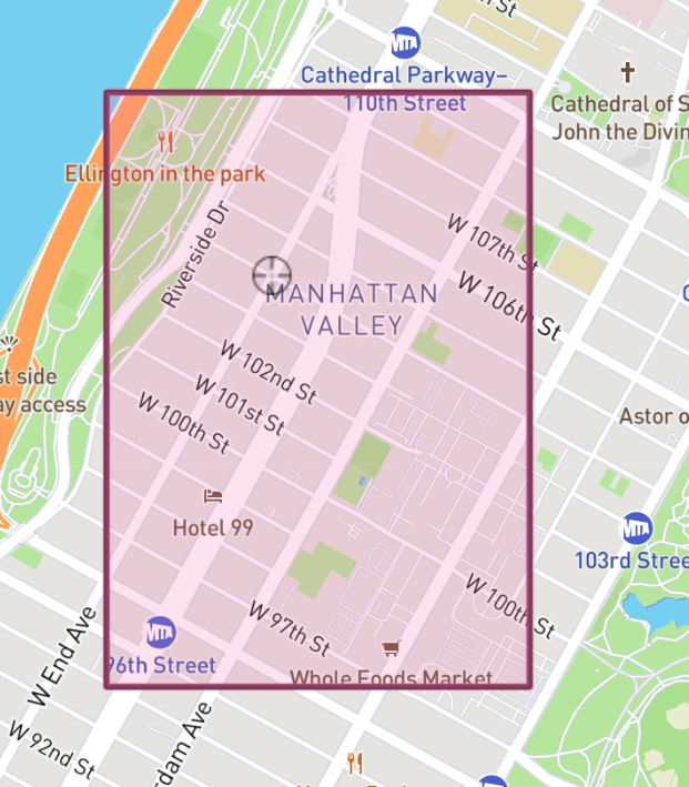
The easiest way to create a scene is using the ​CLI Tool. Scene boundaries are defined by parameterized GPS coordinates. To find these coordinates (either a singular corner or all four), ​bbox is a helpful service. You can zoom and scroll through the world map to find your target area. Once found, the box icon allows you to draw the rectangular area and save the coordinates.

Here, I've generated a set of example coordinates that map a portion of the COSMOS testbed.

-73.973178 40.793488 -73.963824 40.803430

These values can now be used to generate the scene using the CLI tool.

Generating a Coverage Map with Sionna RT

This tutorial is adapted from ​this README and ​this notebook. Feel free to reference either directly if you require custom modifications.

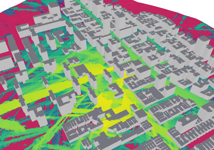
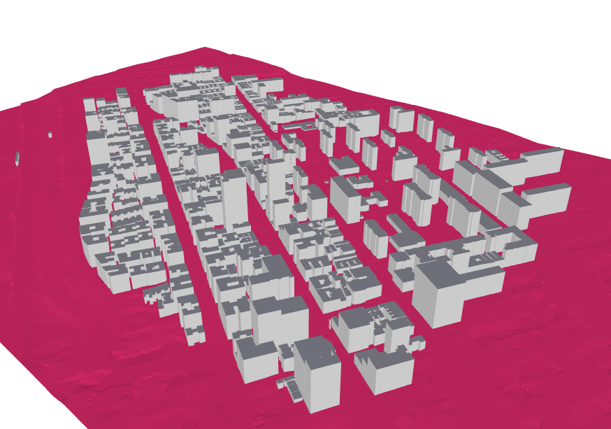
1. In your working directory, use this command to generate the scene. Add LiDAR flag for an accurate, calibrated map terrain:

scenegen bbox -73.973178 40.793488 -73.963824 40.803430 --data-dir scene/COSMOS --enable-lidar-terrain   

2. Add and run core imports:

# Core imports
import numpy as np
import mitsuba as mi
from sionna.rt import load_scene, Transmitter, Receiver, RadioMapSolver, transform_mesh

3. Load and preview your scene:

import os
current_dir = os.getcwd()
print(current_dir)
SCENE_FOLDER = "../scene/COSMOS"
scene = load_scene(f"{SCENE_FOLDER}/scene.xml")

# Interactive 3D visualization and view of the scene
scene.preview();    

You can use the left-click button/scroll wheel to explore the scene.

4. Configure Tx and Rx. This example uses the built-in TR 38.901 Antenna Pattern for transmission at 3.7 GHz. Rx is modeled as an isotropic receiver:

   from sionna.rt import AntennaArray
from sionna.rt.antenna_pattern import antenna_pattern_registry

# Set the operating frequency (n48 band for 5G)
scene.frequency = 3.7e9  # 3.7 GHz

# Define Rx position
ue_position = [20.0, 20.0, 0.0]   # Rx position (x, y, z in meters)

# Define Tx position
gnb_position = [0.0, 0.0, 70.0]

# gNB antenna: 3GPP TR 38.901 pattern (AIRSTRAN D 2200)
gnb_pattern_factory = antenna_pattern_registry.get("tr38901")
gnb_pattern = gnb_pattern_factory(polarization="V")

# Use isotropic antenna pattern
ue_pattern_factory = antenna_pattern_registry.get("iso")
# Polarization should match the transmitter
ue_pattern = ue_pattern_factory(polarization="V")

# SISO: Single antenna element at origin [0, 0, 0] for both TX and RX
single_element = np.array([[0.0, 0.0, 0.0]])  # Shape: (1, 3)

# Configure antenna arrays
scene.tx_array = AntennaArray(
    antenna_pattern=gnb_pattern,
    normalized_positions=single_element.T  # Shape: (3, 1)
)

scene.rx_array = AntennaArray(
    antenna_pattern=ue_pattern,
    normalized_positions=single_element.T  # Shape: (3, 1)
)  

# Create Rx
rx = Receiver(name="ue", position=ue_position, display_radius=0.03)
scene.add(rx)

# Create Tx
tx = Transmitter(name="gnb", position=gnb_position, display_radius=0.03)
scene.add(tx)

5. Generate and Visualize the Coverage Map:

rm_solver = RadioMapSolver()

# Create a measurement surface by cloning the terrain
# and elevating it by 1.5 meters
measurement_surface = scene.objects["ground"].clone(as_mesh=True)
transform_mesh(measurement_surface,
            translation=[0,0,1.5])

rm = rm_solver(scene,
    max_depth=5,
    los=True,
    refraction=False,
    cell_size=(1.0, 1.0),
    size=[1000, 1000],          # Size of the radio map in meters. The number of cells in the x and y directions should be [size/cell_size]
    # orientation=[0, 0, 0],    # Orientation of the radio map plane
    measurement_surface=measurement_surface, # TO BE UDPATED
    # center=[0, 0, 1.5],       # Center of the radio map measurement plane
    precoding_vec=None,
    samples_per_tx=int(1e8)
)

scene.preview(radio_map=rm, rm_db_scale=True, rm_metric="path_gain");   

This example can be modified easily by adjusting the parameters of the Tx/Rx pair. Try it yourself by adjusting their positions by modifying these lines:

# Define Rx position
ue_position = [20.0, 20.0, 0.0]   # Rx position (x, y, z in meters)

# Define Tx position
gnb_position = [0.0, 0.0, 70.0]   

Cite

You've now successfully generated a coverage map using Geo2SigMap and Sionna RT!

If you're able to use the tool as a part of your research, you can use the following citation:

@inproceedings{li2024geo2sigmap,

title={Geo2SigMap: High-fidelity RF signal mapping using geographic databases}, author={Li, Yiming and Li, Zeyu and Gao, Zhihui and Chen, Tingjun}, booktitle={Proc. IEEE International Symposium on Dynamic Spectrum Access Networks (DySPAN)}, year={2024}

}